
Bounding Box 匹配问题探讨
Bounding Box 是常用的 Object Detection 考虑对象而且被越来越多的用在各个学科上。但是,今天在研究的时候发现其实还有一个很细节的小问题是很容易忽略的,这就是如何匹配 Bounding Box 的问题。在这个问题 Computer Vision 和 Physics 的理解有细微的区别,这里记录下。
问题设定
我先讨论下问题设定,我还是用我之前的一个帖子的内容来做例子吧。用矩阵操作快速实现图像识别中 Bounding Box 的准确率和召回率判断,其实这篇文章就是总结下我在那篇博文中的一个失误。在 用矩阵操作快速实现图像识别中 Bounding Box 的准确率和召回率判断 中,我炫技式地使用了 numpy 的操作特性,但是忽略了问题的物理背景。这篇文章纠正下。
假设 predition bounding box number 是 3 个, ground truth bounding box number 是 5 个。
问题解释
在 用矩阵操作快速实现图像识别中 Bounding Box 的准确率和召回率判断 中,我们设定了 IoU_threshold 后其实就是在判断每个预测 BBox 是不是可以实现覆盖上 ground truth BBox。
这里有一个问题,
如果出现两个预测 BBox 都对应同一个 ground truth BBox 那么问题就复杂了,到底哪个是对的?
import numpy as np

# create array data

predict = np.array([[1,2,2,1],
                   [4.5,2.5,10,0.5],
                   [6,6,8,4],
                   [6.26,6.26,8.26,4.26]],np.double)

truth = np.array([[1,4,3,3],
                 [1.2,2.2,2.2,1.2],
                [5,2,8,1],
                [6.1,6.1,8.1,4.1],
                [8.1,8.1,11.1,9.1]], np.double)
# Below is to show the layout of the problem
# red represents truth
# blue represents prediction

import matplotlib.pyplot as plt
import matplotlib.patches as patches
fig = plt.figure()
ax = fig.add_subplot(111, aspect='equal')
recList = list()

# Adding red rectangle from predict
for rect in predict:
    recList.append(
        patches.Rectangle(
            (rect[0], rect[3]),
             np.abs(rect[2] - rect[0]),
             np.abs(rect[3] - rect[1]),
             fill=False,
             edgecolor = "red"
        )
    )

# Adding blue rectangle for truth
for rect in truth:
    recList.append(
        patches.Rectangle(
            (rect[0], rect[3]),
             np.abs(rect[2] - rect[0]),
             np.abs(rect[3] - rect[1]),
             fill=False,
             edgecolor = "blue"
        )
    )

# plot the graph
for p in recList:
    ax.add_patch(p)

plt.text(1.15, 10, "red for precition", size=15, color="red" )
plt.text(1.15, 9, "blue for ground truth", size=15, color="blue" )

plt.plot()
plt.show()
fig.savefig('rect2.png', dpi=300, bbox_inches='tight')
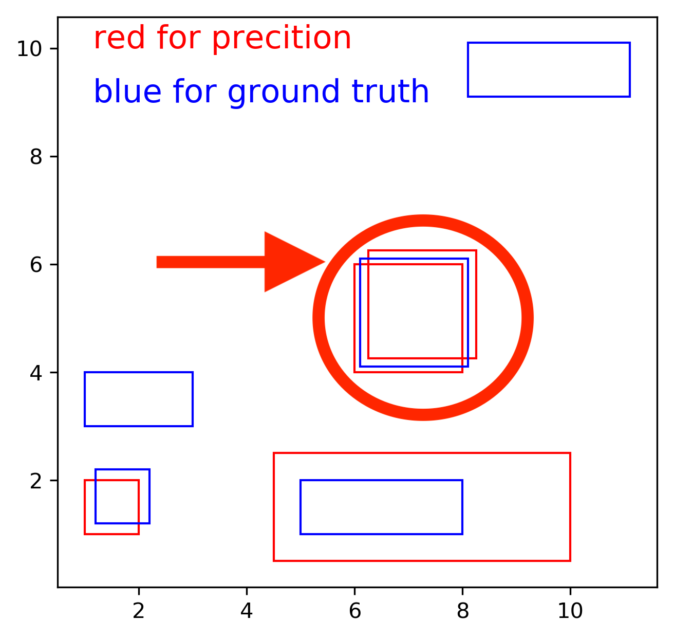
可以看到,在我原来的程序中,这两个 prediction 都是对的,因为在 computer vision 的框架内,我们在评价预测的好坏,单单从预测的角度,这两个评价都是有道理的。所以他们都算对。
但是,在 Physical Reality 的角度,这两个评价只能保留一个,因为如果 gt bbox 已经匹配了一个 prediction,那么它将不能再和别的 pred bbox 匹配。
这两个评价都是对的,因为出发点不同。
需要指明的是
其实实际看,这两个评价框架差距极小,因为在 Object Detection 框架中都有 NMS, non maximum suppression,这个环节,会极大抑制出现上文讨论的两个 pred 对应一个 gt,或者 一个 gt 对应多个 pred 的情况,除非你的图片是 crowded envrionment。
non maximum suppression推荐看这个链接。 Andrew Ng 有很好的解释。
Physical Meaningful Pairing
那么如何实现物理意义上对的gt bbox 和 pred bbox 匹配呢?
其实主要方法也很简单,
- 构建 IoU Performance Matrix,其中每一个 行 代表 pred,列 代表 gt
- 从 IoU Performance Matrix 中最大的 value 开始匹配,每匹配成功一个 value,这代表这个 value 大于我们设定的 IoU_theshold,就记录相应的匹配,同时将该 value 对应的 行 和 列 都设置为 0,这代表他们永远不可能再被使用,因为 IoU 的最小值就是 0,代表没有任何交集。
我直接上程序吧,这里有几个 varibale setting 在前面。
当然 IoU 计算也是常用的知识点,我这里直接拷贝下别处的标准答案 常考题 IoU 计算
# boxA 存储的是边界框的左上顶点坐标和右下顶点坐标
# boxA=[x1,y1,x2,y2]
def iou(boxA, boxB):
    # 计算重合部分的上下左右4个边的值,注意最大最小函数的使用
    left_max = max(boxA[0],boxB[0])
    top_max = max(boxA[1],boxB[1])
    right_min =  min(boxA[2], boxB[2])
    bottom_min = min(boxA[3], boxB[3])

    # 计算重合部分的面积
    inter = max(0,(right_min-left_max)) * max(0, (bottom_min-top_max)) # 宽*高
    Sa = (boxA[2]-boxA[0])*(boxA[3]-boxA[1])
    Sb = (boxB[2]-boxB[0])*(boxB[3]-boxB[1])

    # 计算所有区域的面积并计算 iou
    union = Sa+Sb-inter
    iou = inter/union
    return iou
算法如下,需要注意,col 没有便捷的操作,所以需要一个 loop
import numpy as np

# create array data

predict = np.array([[1,2,2,1],
                   [4.5,2.5,10,0.5],
                   [6,6,8,4],
                   [6.26,6.26,8.26,4.26]],np.double)

truth = np.array([[1,4,3,3],
                 [1.2,2.2,2.2,1.2],
                [5,2,8,1],
                [6.1,6.1,8.1,4.1],
                [8.1,8.1,11.1,9.1]], np.double)
# get useful variables
nums_pred = len(predict)
nums_gt = len(truth)

iou_matrix = np.zeros((nums_pred,nums_gt))


# boxA 存储的是边界框的左上顶点坐标和右下顶点坐标
# boxA=[x1,y1,x2,y2]
def iou(boxA, boxB):
    # 计算重合部分的上下左右4个边的值,注意最大最小函数的使用
    left_max = max(boxA[0],boxB[0])
    top_max = max(boxA[1],boxB[1])
    right_min =  min(boxA[2], boxB[2])
    bottom_min = min(boxA[3], boxB[3])

    # 计算重合部分的面积
    inter = max(0,(right_min-left_max)) * max(0, (bottom_min-top_max)) # 宽*高
    Sa = (boxA[2]-boxA[0])*(boxA[3]-boxA[1])
    Sb = (boxB[2]-boxB[0])*(boxB[3]-boxB[1])

    # 计算所有区域的面积并计算 iou
    union = Sa+Sb-inter
    iou = inter/union
    return iou

def transformBBox(boxA):
	# 将 BBox 从左下 + 右上 表示转换为 左上 + 右下
	return [boxA[0], boxA[3], boxA[2], boxA[1]]
# get iou matrix

for i in range(nums_pred):
	for j in range(nums_gt):
		#print(truth[j])
		iou_matrix[i][j] = iou(transformBBox(predict[i]), transformBBox(truth[j]))

print(iou_matrix)

res  = []
IOU_theta = 0.4

while np.any(iou_matrix > IOU_theta):
	ind = np.argmax(iou_matrix)
	ind_col = ind % nums_gt
	ind_row = (ind - ind_col) // nums_gt
	print("row = %d, col = %d"%(ind_row, ind_col))
	# store results for more analysis
	res.append([predict[ind_row], truth[ind_col]])
	# set the correspoding row and col to zero
	# exclude those already paired from future comparsion
	iou_matrix[ind_row][:] = 0
	# set col to 0
	for ii in range(nums_pred):
		iou_matrix[ii][ind_col] = 0
	print(iou_matrix)
print(res)
当然,这个算法有一个限制,那就是最好的 Precision 和 Recall 其实取决于你的 prediction 和 gt BBox 的数目。
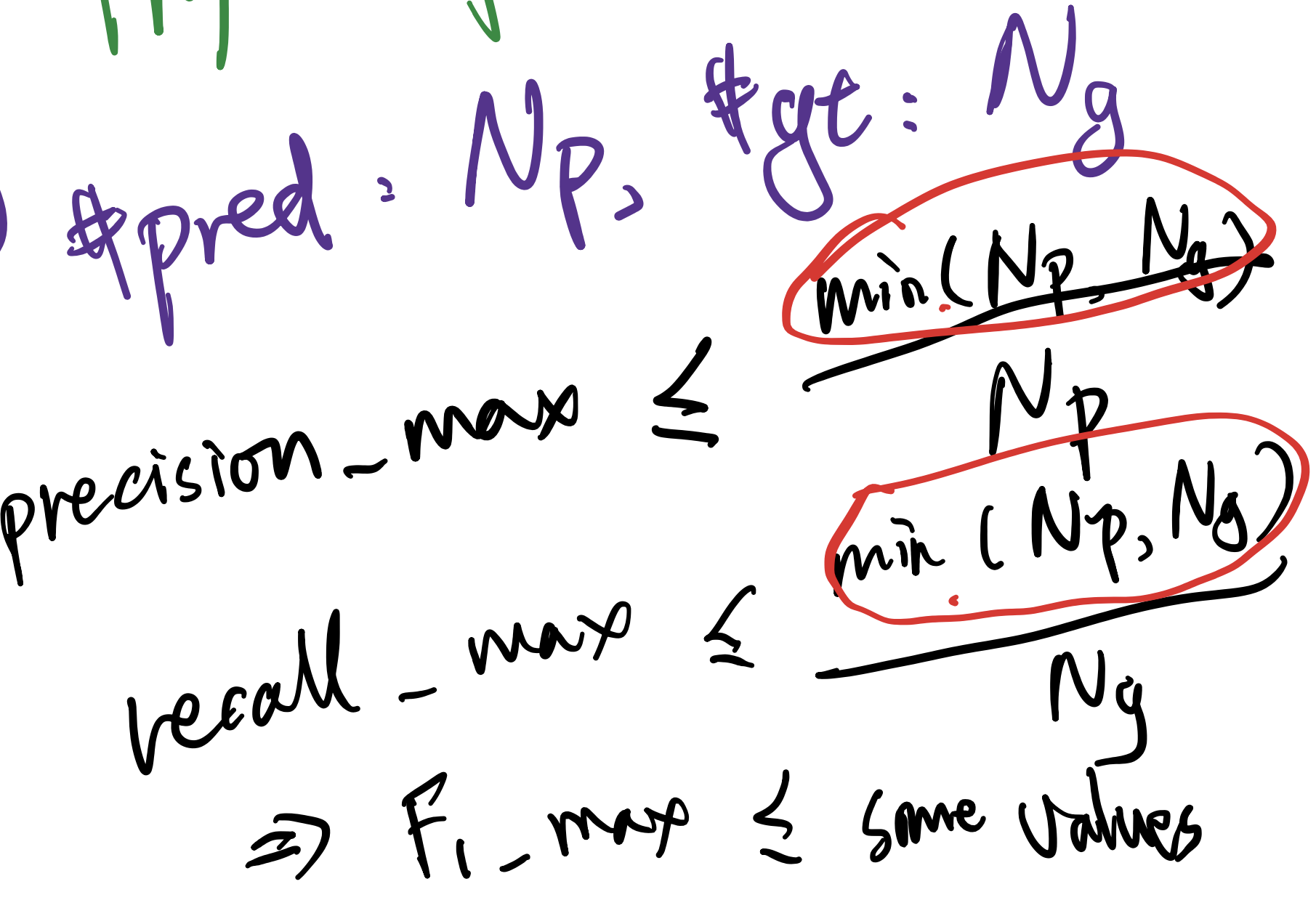
当然这个也是合理,如果你的模型固定了,你的 output 固定,你的 performance 也需要固定。
同时这样也要求你控制 pred 的数目,最后达到最好的效果。只有在 pred 数目 和 gt 数目相等的情况下,才有可能 P,R 都到 1。
总结
这其实是一个特别细节的问题,但是仔细思考下才发现也非常有意思。
这也是别人会问你们这些具体领域应用 CV 的人和 CV 有什么区别的时候的一个例子, CV 是基础,但是也要考虑到具体的学科的细节。