Ising相变的模拟

起因

这是上学期的一个Project，似乎不应该现在才放出来。但是老师一直没有给分，因为是论文的一部分，全文发上来万一来个查重什么。所以等到老师终于给分了，就直接贴上来了。

这是一份英文的报告。

Latex转过来的时候的参考文献格式我就没怎么换，都放在最后了。

abstract

In this lab experiment, we use importance sampling Monte Carlo techniques to study $60 \times 60 $ 2-D Ising Model. We will further discuss the thermal properties of Ising Model.

Introduction

Ising Model is one of the most important the theoretical model in statistical physics,which is proposed first to explain the start of ferro-magnetism. The central thought of Ising Model is representing real system like magnetic Curie points or order-disorder phenomena transitions in alloy as molecules interacting with nearest neighbour in a lattice \cite{Rev}. Although Ising Model was scorned and ignored by most scientists during its early ages \cite{Rev}, it has gained more and more popularity in the science community for both its multi-disciplines application in physics, chemistry, metallurgy,and mathematics and its simple and elegant lattice models physical intuition.

Ising Model can be simply described as the lattice model with $-1$ or $+1$ spins constrained to the site of lattice and spin interactions only exist between nearest neighbours.

1-D Ising Model is proposed and solved by Krnst Ising and his PhD supervisor Wilhelm Lenz and their result shows there is no phase transition \cite{Rev}. However, it is until 1944, Onsager obtained exact results of 2-D Ising Mode and the analysis shows that there is a second order phase transition \cite{guide}. But 3-D Ising Model is still no exact solution.

In this report, we will generally focus on 2-D Ising Model and the lattice size is $60 \times 60$ and the temperature will be decreased from 3.5 to 1.5 by step 0.1 ,then increased form 1.5 to 3.5

Algorithm

Generally we simulate Ising Model following the rule of importance sampling which only counts those configurations that contribute greater to the final state of system.

To realize this, we use Metropolis Method. In the classic, Metropolis Method generates configuration form the previous state using the energy difference dependent transition probability which means that the new state can be produced by old state multiplies the transition probability. This procedure can be described by a master equation:

\[\frac{\partial P_n(t)}{\partial t}=-\sum_{n \neq m}[P_n(t)W_{n \rightarrow n } - P_m(t)W_{m \to n} ]\]

where $P_n(t)$ is the probability of the system being in state n at time, and $W_{n \to m }$ is the transition rate for $ n \to m$.

In equilibrium, we get $\frac{\partial P_n(t)}{\partial t} =0 $ and this means that the right two terms of equation \eqref{masterequ} is equal which gives

\[P_n(t)W_{n \rightarrow n }=P_m(t)W_{m \to n}\]

And based on the knowledge of Statistical Physics we can know that the probability of n state occurring in a classical system is given by:

\[P_n(t)=e^{-E_n/k_BT}/Z\]

where Z is the partition function.

However, we actually know little of the system’s partition function. To avoid this difficulty, we generate each new state directly from the preceding state and repeating this we get a Markov Chain of states. So if we produce the n state form m state, the relative transition probability will only depends on the energy difference between the two states which is :

\[\Delta E= E_n - E_m\]

So the uncertain partition function cancels.

Any transition rate satisfying detailed balance is acceptable in Monte Carlo Simulation. And in this case, we use Metropolis Scheme is

\[W_{n \to m} = \left\{ \begin{matrix} \tau_0^{-1} \exp(-\Delta E/ k_BT), & \Delta E > 0\\ \tau_0^{-1}, & \Delta E<0 \end{matrix} \right.\]

where $\tau_0$ is the time required to attempt one move form old state to new state which is a spin-flip action in Ising Model.

So we can describe Metropolis Importance Sampling Motel Carlo Scheme as following :

Choose an initial state
Choose a site i
Calculate the energy change $\Delta E$ which results from if the spin at site i is overturned
Generate a random number r that $0<r<1$
Go the next site and go to step 3
After enough steps, sample needed physical prosperities

In the simulation, we use the reduced unit to simply the calculation and shorten the time of computing.

Generally, we make that the unit of energy is $J$, the unit of length is 1 and unit of mass is also 1. In this unit system, temperature is $J/k_B$,where $k_B$ is the Boltzmann constant. If we want to further simply the unit system, we can set $J=1$, so that the temperature is in unit of $1/k_B$.

##Calculating Observables

After we have set up the scheme for the The Metropolis Algorithm, we further discuss the observables or those physics quantities we are interested in.

We know that the expectation value of an observable A can be written as:

\[\left \langle A \right \rangle=\frac{\sum_r A_re^{-\beta E_r}}{\sum_r e^{\beta E_r}}\]

where $A_r$ is the value of A for the state r and $E_r$ is the energy for the state r.

And using The Metropolis Algorithm, we can get many interesting prosperities about the system.

For system energy $E$ we have

\[E=-J \sum_{i,j} S_i S_j\]

where $J$ is the interaction constant between the neighbour spins.

For magnetization, we have

\[M= \sum_{i}^{N} S_i\]

where $N$ is the total number of the spins.

For specific heat, we have:

\[C_v=\frac{\partial E}{\partial T}=-\frac{\beta}{T}\left[\left \langle E^2 \right \rangle -\left( \left \langle E \right \rangle \right)^2 \right]\]

Incidentally, this is known as the Fluctuation Dissipation Theorem.

Also for magnetic susceptibility, $\chi $, can be written in terms of the variance in the magnetization:

\[\chi=\frac{\partial \left \langle M \right \rangle}{\partial H}=\beta\left[\left \langle M^2 \right \rangle -\left( \left \langle M \right \rangle \right)^2 \right]\]

So we need to keep record of $E, E^2 , M , $ and $M^2$ , we can get the evolution of the energy, the magnetization, the specific heat, and the magnetic susceptibility.

Algorithm Details

During the program of Monte Carlo Simulation, there are generally two details needed to pay attention to. The first one is how to calculate energy difference between the old state and new one.The second one is how to realize periodic boundary conditions.

Calculating Energy Difference

If we just use the common method to calculate the energy changes, the amount of calculations will be huge but if we further explore the different cases in energy changes there are only 5 results will happen if we change the spin of one site.

tu1

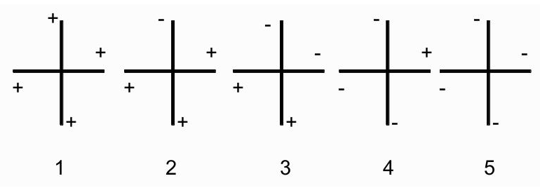
Now if we assume that we have get one site $(i,j)$ to change its spin, first we make it has spin $-1$. So if it were overturned, the spin is $+1$.Now considering its nearest four neighbours it will be only 5 cases if you take symmetry into consideration. The 5 cases are like figure \ref{5case} has shown.

So we can get a table of energy changes as table \ref{energychangeminus}, here we use the symbol $+$ and $-$ to represent up and down spin. Following the same routine, we can get the energy changes of up spin as table \ref{energychangeup}

tu1

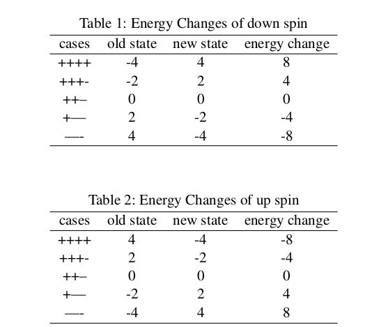
Based on table \ref{energychangeminus} and table \ref{energychangeup}, we can conclude that the energy change of turning site $(i,j)$ is equation \eqref{engchange}:

\[\Delta E = 2S_i \sum_{n.n(j)}S_j\]

where $n.n$ means the nearest four neighbours of site $(i,j)$.

Periodic Boundary Conditions

Because our simulations are performed on infinite systems, so we must take the effect of those edges and surfaces into consideration because they may be different from those in the body or inner part of the system. We can effectively eliminated these boundaries by wrapping the $N \times N$ Ising lattice on a the $ (N+1) \times (N+1)$ one.

The common periodic boundary conditions may be like this:

tu1

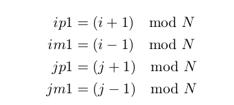
where $ip1,im1,jp1,jm1$ means plus and minus 1 form i and j and $\mod$ means modular arithmetic and L is the size of the lattice.

But this involves too many computations for $mod$ can not be computed easily. But we can referred to two tables to simply the calculation for periodic boundary condition only happens on the edges of lattice, which means that the index of one spin site $(i,j)$ must have this relations:$i=1 , i= L$ or $j= 1 , j= L$.So we can calculated those periodic boundary conditions before which can also fasten the simulation.

Conclusion

After doing all the simulation work, we will further discuss the propensities of Ising Model.

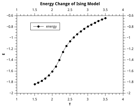
###Observables Calculation As figure \ref{energy} has shown, energy is a continuous function of temperature, which, as we expect, increases as a function of T .

tu1

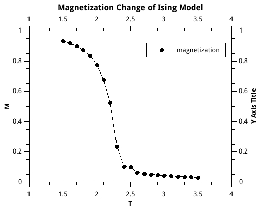
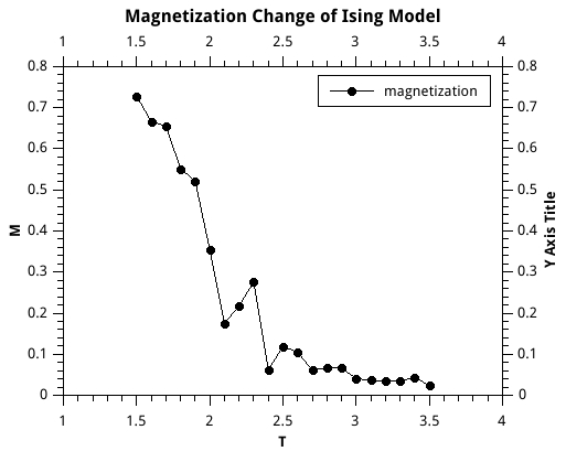
As figure \ref{mag} has shown, magnetization drops off sharply near the critical temperature, which, in our units where k = J = 1, is approximately 2.3.

tu1

As figure \ref{sheat} has shown, specific heat has a peak at the critical temperature.

tu1

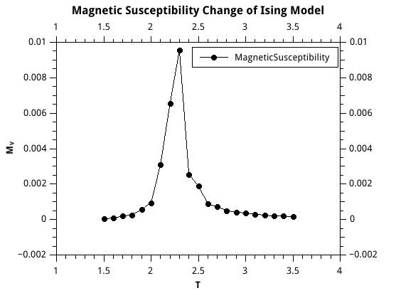
As figure \ref{magv} has shown,magnetic susceptibility has a sharp jump at the critical temperature.

tu1

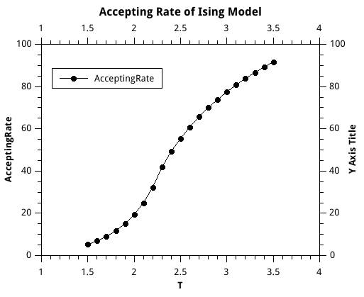
Average Accepting Rate

And in figure \ref{acrate} we show the change of accepting rate. We can easily find out that the accepting rate increases when temperature does. This is just what we except. When temperature increases, a single site overturn will be less important to the change of system energy or we can say when temperature increases, the spins will be more disordered than they are at low temperature. At low temperature, all the spins are like frozen at their own site and less likely to change their direction.

tu1

Phase Transition

tu2

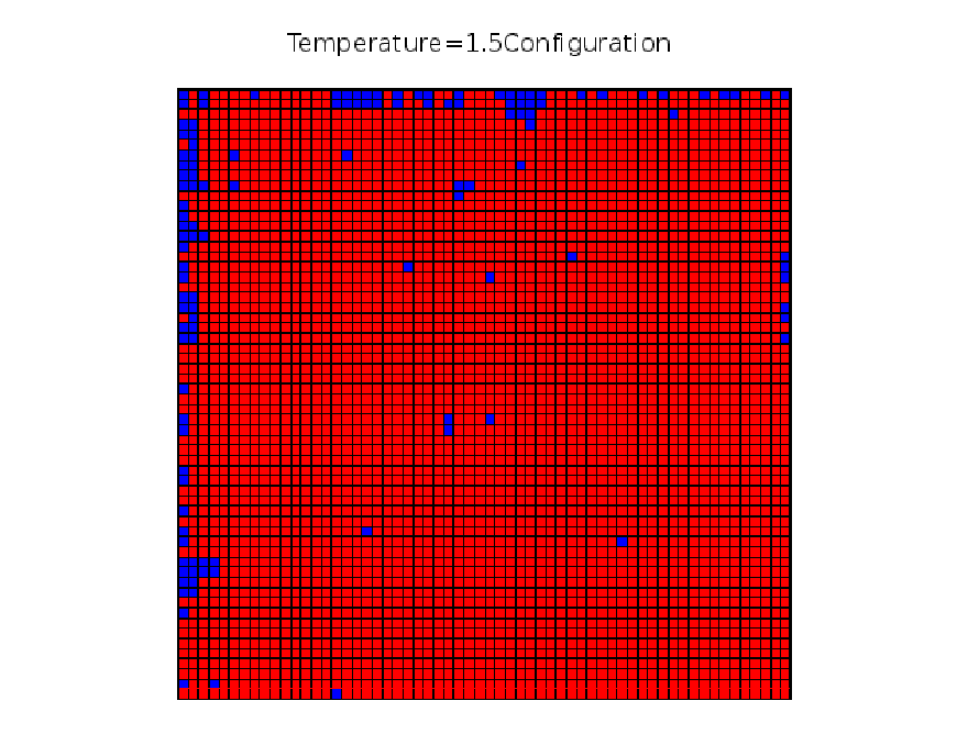
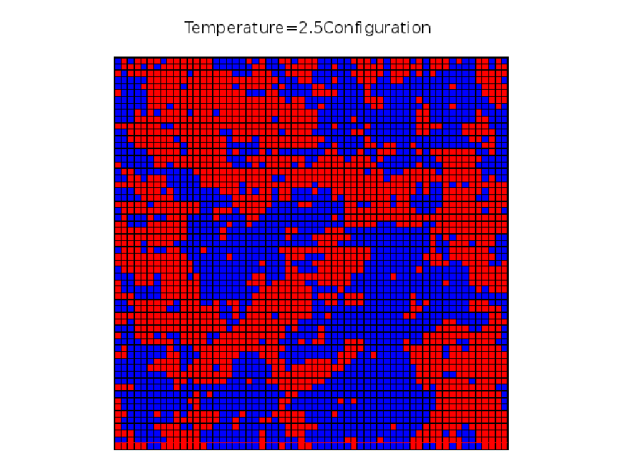
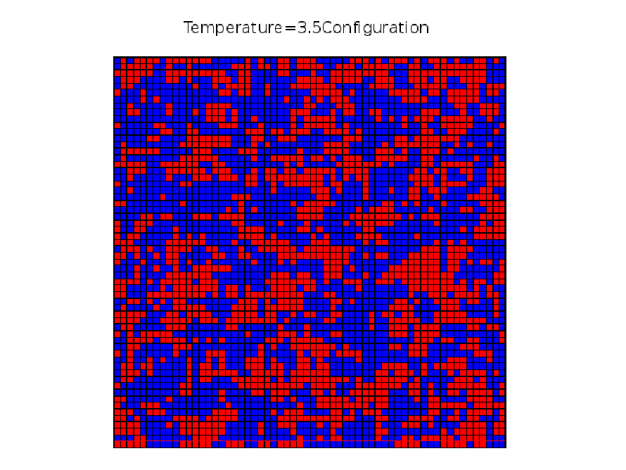
Then in figure \ref{transfer} we show the phase transition in Ising Model. In figure \ref{transfer} from top to bottom, temperature goes from 3.5 to 1.5.

Following we will show three key the configuration of three states at temperature 3.5, 2.5 ,1.5 in figure \ref{configure}

tu2

Equilibrium Time

In my simulation, I set $40 \% $ of the total Monte Carol Move to be the equilibrium stage. And this seems works fine when I set $mc_ total_steps=50000000$ which means the program will try to overturn the spin of Isng Model Lattice 50000000 times.

But if the $mc_ total_steps$ is less the result’s accuracy will suffer.For example figure \ref{mag500000} is the magnetization change of $mc_ total_steps=500000$.

tu2

If you compare figure \ref{mag500000} with figure \ref{mag} you will find that figure \ref{mag} is much better. And nonetheless to say, specific heat, the image is wrong if mc_ total_steps is low which also means not enough equilibrium time.

###Correlation Generally speaking, there are two kinds of correlations existing in Ising Model: one is time correlation, the other is space correlation. Below we will focus on both two kinds.

Time Correlation

As we use Monte Carlo Step Time as the unit of our simulation time unit, so time correlation can be also explained as the Monte Carlo Move Step Correlation.So different numbers of simulation steps can result different result which has been explained in previous section \ref{equ} Equilibrium Time.

Space Correlation

Because a change of one spin site may result another change of another spin site, we can define a correlation length to represent this effect, which is also known as space correlation. So if the distance of two spin sites is within correlation length we think they are coupled or interacted and if not, we ignore their correlation.

In theory, we can define correlation between two spin sites as:

\[Cor = \left \langle (S_i - \left \langle S_i \right \rangle )( S_j - \left \langle S_j \right \rangle ) \right \rangle = \left \langle S_i S_j \right \rangle - \left \langle S_i \right \rangle \left \langle S_j \right \rangle\]

And one can easily guess correlation between two spin sites must be related with the distance of two spin sites and may also be related with temperature.To be simple, I choose spin site$(30,30)$ and its neighbours $(31,31),(34,34),(37,37),(40,40),(43,43)$ to calculate their correlation and show their relation ship of distance and temperature.

The result is figure \ref{corr} has shown.

tu2

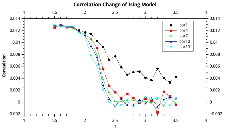
We can see that when the temperature is high, the correlation is weak but when temperature approximates the critical temperature where phase transition happens the correlation jumps up quickly. So we can say that phase transition is closely related with correlation between different spins. Also figure \ref{corr} tells us that at a specific temperature the nearer the stronger correlation . If we want to define some correlation length of spin sites, it seems that we can set the correlation length between $2 \sim 3$ at high temperature. And at low temperature,correlation length is less obvious for the very strong correlation interaction.

Initial Conformation dependence

Based on my study, I think initial conformation is useless for the final result of Ising Model if you set a large enough total number of simulation steps. But I do agree, that initial conformation can influence the equilibrium time and large enough total number of simulation steps can cancel its effect.

Programme Code

!**********************************************************************
!The programe performs Motel Carlo Simulation for 2D Ising Model.
!**********************************************************************
program main

implicit none

! Parameter declarations:
integer,parameter :: nrow=60
integer,parameter :: ncol=60
integer,parameter :: mc_total_steps=50000000
integer,parameter :: mc_eq_steps=20000000
integer,parameter :: mc_sample_steps=50000
real,parameter    :: maxtemperature=3.5         
real,parameter     :: mintemperature=1.5
real,parameter     :: deltatemperature=0.1

! Variable declarations:
integer             :: A(nrow,ncol)   
integer             :: ip(60),im(60),jp(60),jm(60)
integer             :: i
integer             :: j
integer             :: mc_counting
integer             :: mc_success_move
integer             :: samplenum

real                :: RanNum
real                :: Tnow

character(len=70) :: filename
character(len=70) :: captionname

!Sample Variable declarations:
real                :: energysum
real                :: energy2sum
real                :: mangentsum
real                :: mangent2sum
real                :: energysumtemp
real                :: energy2sumtemp
real                :: mangentsumtemp
real                :: mangent2sumtemp





!-----------------Initialization--------------------------------------------------!
do i =1,nrow
    do j=1,ncol
        call random_number(RanNum)
        if(RanNum >= 0.5) then
            A(i,j)=1
        else
            A(i,j)=-1
        end if


    end do
end do

call plot_file ( nrow, ncol, A, 'Initial Configuration', 'ising_2d_initial.txt', &
    'ising_2d_initial.png' )
!calculate the call peridoic boundary condition(ip,im,jp,jm)
call peridoicboundary(ip,im,jp,jm)

!-----------------MCSimulation and Sampleing------------------------!
	 Tnow=maxtemperature
	 
 do  while(Tnow>=mintemperature)
	 mc_counting=0
	 mc_success_move=0
	 energysum=0
	 energy2sum=0
 	 mangentsum=0
	 mangent2sum=0
	 samplenum=0

	  
	 write(*,*) Tnow

	do while(mc_counting<= mc_total_steps)
		call mc_onestep_move(A,ip,im,jp,jm,Tnow,mc_success_move)
		mc_counting=mc_counting+1
		if((mc_counting > mc_eq_steps) .and. (MOD(mc_counting,mc_sample_steps)==0))	then
			mangentsumtemp=0
			energysumtemp=0
			energy2sumtemp=0
			mangent2sumtemp=0
			
			do i =1,nrow
				do j=1,ncol
				mangentsumtemp=mangentsumtemp+A(i,j)
				energysumtemp=energysumtemp+(A(ip(i),j)+A(im(i),j)+A(i,jp(j))+A(i,jm(j)))*A(i,j)*(-0.5)
				end do
			end do
			mangentsum=mangentsum+abs(mangentsumtemp/3600.0)
			energysum=energysum+energysumtemp/3600.0
			 
			
            energy2sumtemp=(energysumtemp/3600.0)**2
			mangent2sumtemp=(abs(mangentsumtemp/3600.0))**2
			energy2sum=energy2sum+energy2sumtemp
			mangent2sum=mangent2sum+mangent2sumtemp
			 

			samplenum=samplenum+1
			 
		else 			  
		end if
     
	end do	
!------------------------saving result-------------------------------------------!
 
	  
  if (Tnow<=1.0) then  
  write (filename, '("plotdata0", F2.1)' )  Tnow
  else
  write (filename, '("plotdata", F3.1)' ) Tnow
  end if
  open (file='resulrsummary.txt',unit=16,position='append')
  write (16,*) & 
  Tnow,mc_success_move,mangentsum/samplenum,mangent2sum/samplenum,energysum/samplenum,energy2sum/samplenum
  close (16)
  if (Tnow<=1.0) then  
  write (captionname, '("Temperature=0", F2.1)' )  Tnow
  else
  write (captionname, '("Temperature=", F3.1)' ) Tnow
  end if
  call plot_file ( nrow, ncol, A, trim(captionname)//'Configuration', trim(filename)//'.txt', &
     trim(filename)//'.png' )
   
!-----------------Next temperature------------------------!

Tnow=Tnow-deltatemperature	
end do

write(*,*) 'Done!'
end program



subroutine peridoicboundary(ip,im,jp,jm)
!*****************************************************************************80
!this subroutine caculate the peridoic boundary conditions for simulation
!
integer :: i
integer :: ip(60),im(60),jp(60),jm(60)

do i=1,60
	ip(i)=i+1
	im(i)=i-1
	jp(i)=i+1
	jm(i)=i-1
end do
ip(60)=1
im(1)=60
jp(60)=1
jm(1)=60
end


subroutine mc_onestep_move(M,xp,xm,yp,ym,T,mc_success_move)
!*****************************************************************************80
!this subroutine perform one move of Monte Carlo setp which also means turn one
!site of Ising Model up or down against the previous state. Then we caculate the 
!energy difference to determine whether this move is accepted or not.
! 
implicit none
real    :: x
real    :: y
real    :: energy_difference
real    :: neighbour_spin_sum
real    :: pro
real    :: T
real    :: judgement
integer :: mc_success_move
integer :: M(60,60) 
integer :: xp(60),xm(60),yp(60),ym(60)
integer :: xint
integer :: yint
call random_number(x)
call random_number(y)
xint=int(60*x)
yint=int(60*y)
if(xint==0) then
xint=1
else 
end if
if(yint==0) then
yint=1
else
end if

neighbour_spin_sum=M(xp(xint),yint)+M(xm(xint),yint)+M(xint,yp(yint))+M(xint,ym(yint))
energy_difference=(2)*M(xint,yint)*neighbour_spin_sum
pro=exp((-1)*energy_difference/T)

call random_number(judgement)
If (judgement<pro) then
	M(xint,yint)=(-1)*M(xint,yint)
	mc_success_move=mc_success_move+1
else
	continue
end if
end



subroutine plot_file ( m, n, c1, title, plot_filename, png_filename )

!*****************************************************************************80
!
!! PLOT_FILE writes the current configuration to a GNUPLOT plot file.
!
!  Licensing:
!
!    This code is distributed under the GNU LGPL license.
!
!  Modified:
!
!    29 June 2013
!
!  Author:
!
!    John Burkardt
!
!  Parameters:
!
!    Input, integer ( kind = 4 ) M, N, the number of rows and columns.
!
!    Input, integer ( kind = 4 ) C1(M,N), the current state of the system.
!
!    Input, character ( len = * ) TITLE, a title for the plot.
!
!    Input, character ( len = * ) PLOT_FILENAME, a name for the GNUPLOT
!    command file to be created.
!
!    Input, character ( len = * ) PNG_FILENAME, the name of the PNG graphics
!    file to be created.
!
  implicit none

  integer ( kind = 4 ) m
  integer ( kind = 4 ) n

  integer ( kind = 4 ) c1(m,n)
  integer ( kind = 4 ) i
  integer ( kind = 4 ) j
  character ( len = * ) plot_filename
  integer ( kind = 4 ) plot_unit
  character ( len = * ) png_filename
  real ( kind = 8 ) ratio
  character ( len = * ) title
  integer ( kind = 4 ) x1
  integer ( kind = 4 ) x2
  integer ( kind = 4 ) y1
  integer ( kind = 4 ) y2

  call get_unit ( plot_unit )

  open ( unit = plot_unit, file = plot_filename, status = 'replace' )

  ratio = real ( n, kind = 8 ) / real ( m, kind = 8 )

  write ( plot_unit, '(a)' ) 'set term png'
  write ( plot_unit, '(a)' ) 'set output "' // trim ( png_filename ) // '"'
  write ( plot_unit, '(a,i4,a)' ) 'set xrange [ 0 : ', m, ' ]'
  write ( plot_unit, '(a,i4,a)' ) 'set yrange [ 0 : ', n, ' ]'
  write ( plot_unit, '(a)' ) 'set nokey'
  write ( plot_unit, '(a)' ) 'set title "' // trim ( title ) // '"'
  write ( plot_unit, '(a)' ) 'unset tics'

  write ( plot_unit, '(a,g14.6)' ) 'set size ratio ', ratio
  do j = 1, n
    y1 = j - 1
    y2 = j
    do i = 1, m
      x1 = m - i
      x2 = m + 1 - i
      if ( c1(i,j) < 0 ) then
        write ( plot_unit, '(a,i3,a,i3,a,i3,a,i3,a)' ) 'set object rectangle from ', &
          x1, ',', y1, ' to ', x2, ',', y2, ' fc rgb "blue"'
      else
        write ( plot_unit, '(a,i3,a,i3,a,i3,a,i3,a)' ) 'set object rectangle from ', &
          x1, ',', y1, ' to ', x2, ',', y2, ' fc rgb "red"'
      end if
    end do
  end do

  write ( plot_unit, '(a)' ) 'plot 1'
  write ( plot_unit, '(a)' ) 'quit'

  close ( unit = plot_unit )

  write ( *, '(a)' ) ' '
  write ( *, '(a)' ) '  Created the gnuplot graphics file "' // trim ( plot_filename ) // '".'

  return
end

subroutine get_unit ( iunit )

!*****************************************************************************80
!
!! GET_UNIT returns a free FORTRAN unit number.
!
!  Discussion:
!
!    A "free" FORTRAN unit number is a value between 1 and 99 which
!    is not currently associated with an I/O device.  A free FORTRAN unit
!    number is needed in order to open a file with the OPEN command.
!
!    If IUNIT = 0, then no free FORTRAN unit could be found, although
!    all 99 units were checked (except for units 5, 6 and 9, which
!    are commonly reserved for console I/O).
!
!    Otherwise, IUNIT is a value between 1 and 99, representing a
!    free FORTRAN unit.  Note that GET_UNIT assumes that units 5 and 6
!    are special, and will never return those values.
!
!  Licensing:
!
!    This code is distributed under the GNU LGPL license.
!
!  Modified:
!
!    26 October 2008
!
!  Author:
!
!    John Burkardt
!
!  Parameters:
!
!    Output, integer ( kind = 4 ) IUNIT, the free unit number.
!
  implicit none

  integer ( kind = 4 ) i
  integer ( kind = 4 ) ios
  integer ( kind = 4 ) iunit
  logical lopen

  iunit = 0

  do i = 1, 99

    if ( i /= 5 .and. i /= 6 .and. i /= 9 ) then

      inquire ( unit = i, opened = lopen, iostat = ios )

      if ( ios == 0 ) then
        if ( .not. lopen ) then
          iunit = i
          return
        end if
      end if

    end if

  end do

  return
end

Reference

\bibitem{Rev} Brush S G. History of the Lenz-Ising model[J]. Reviews of Modern Physics, 1967, 39(4): 883.

\bibitem{guide} Landau D P, Binder K. A guide to Monte Carlo simulations in statistical physics[M]. Cambridge university press, 2009,P68.

\bibitem{john} John Burkardt,Monte Carlo 2D Ising Model Fortran90 Code,\url{http://people.sc.fsu.edu/~jburkardt/f_src/ising_2d_simulation/ising_2d_simulation.html}

Written on May 11, 2014